|
Physical principles of DC resistivity |
IntroductionThis chapter presents the important phyiscal principles upon which DC resistivity methods are based. The relations between current flow, potentials and resistivity in uniform ground are explained. This forms the basis for the concept of apparent resistivity derived from practical survey arrangements (two current and two potential electrodes planted at the surface). The effect of anisotropic ground upon measured potentials is then described. Finally, charge distribution is explained because it is a useful way of understanding how potentials arise at the surface due to variations in electrical conductivity underground. The forward modeling relations are also based upon charge distribution.
|
 |
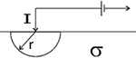 |
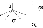
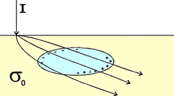
Consider first a uniform Earth and one electrode, which is pumping a current, I, into the ground. We want to find the electric potential within the ground at a distance, r, from the current source. The current density in the ground is related to source current injected, and the potential measured at a surface defined by, r, is related to the electric field that exists in the ground because of the current which flows radially outward from its point source. These two relations will be combined with the 3D form of Ohm's law to end up with an expression for conductivity (the physical property we want) in terms of the current source, measured potential, and the distance.
First, by symmetry the current density out of the hemisphere of radius, r, is
and the current is flowing in a radial direction. Since J=![]() E (Ohm's Law), the electric field must also be pointing radially outward. The relationship between the electric field and the potential is
E (Ohm's Law), the electric field must also be pointing radially outward. The relationship between the electric field and the potential is
Combining the expression for E, Ohm's Law and equation 1, we have
If we intergrate,
So the potential due to a point current electrode at the surface is:
.
The electric potential inside the earth caused by the radial flow of current is illustrated in the diagram below.
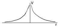
At the surface, where measurements are made, the potential is infinite at the current electrode because r=0, and it decays with distance.
 |
 In a geophysical survey, current is injected into the ground using two electrodes. It is convenient to label the electrodes as
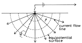
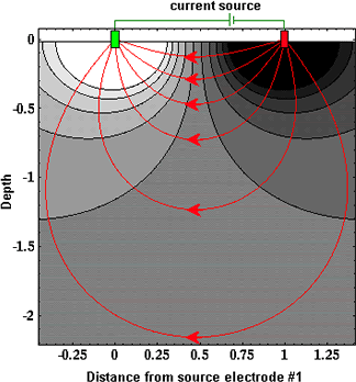 For a uniform Earth, lines of current flow are shown in red in the figure to the right, and corresponding lines of equal potential (equipotential lines) are shown in black. Instead of the current flowing radially out from the current electrodes, it now flows along curved paths connecting the two current electrodes. Six current paths are shown. Between the surface of the earth and any current path we can compute the total proportion of current encompassed. The table below shows the proportion for the six paths shown (current path 1 is the top-most path and 6 is the bottom-most path).
| Current Path | % of Total Current |
|---|---|
| 1 | 17 |
| 2 | 32 |
| 3 | 43 |
| 4 | 49 |
| 5 | 51 |
| 6 | 57 |
From these calculations and the graph of the current flow shown above, notice that almost 50% of the current placed into the ground flows through rock at depths shallower than or equal to the current electrode spacing.
The graph shown below plots the potential that would be measured along the surface of the earth for a fixed 2-electrode source. The voltage we would observe with our voltmeter (between purple electrodes) is the difference in potential at the two voltage electrodes, ΔV.
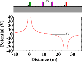
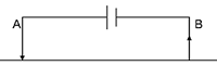
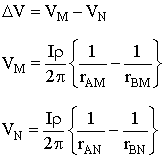
If there are two current (source) electrodes, the potential is the superposition of the effects from both. In a practical experiment (figure below), one electrode, A, is the positive side of a current source, and the other electrode, B, is the negative side. The current into each electrode is equal, but of opposite sign. For a practical survey, we need two electrodes to measure a potential difference. These are M, the positive terminal of the voltmeter (the one closest to the A current electrode), and N, the negative terminal of the voltmeter.
The measured voltage is a potential difference (VM - VN) in which each potential is the superposition of the effects from both current sources:
 |
... so ... |
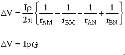 |
In the final relation, G is a geometric factor which depends upon the geometry of all four electrodes. Finally, we can define apparent resistivity (discussed in the measurements section) by rearranging the last expression to give:
. Similarly, the apparent conductivity is,
.
We use the term apparent resistivity because it is a true resistivity of materials, only if the Earth is a uniform halfspace within range of the survey. Otherwise, this number represents some complicated averaging of the resistivities of all materials encountered by the current field.
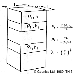
Structural anisotropy (for example, layering or fracturing) causes the simple form of Ohm's law to break down because current flow is not necessarily parallel to the forcing electric field. Instead of simply writing ![]() , we have to write
, we have to write
.
In homogeneous ground with single current and potential electrodes, the expression for V (voltage) in terms of resistivity and distance from the current source is ![]() (which was shown above). In anisotropic ground, there are different values of resistivity for the horizontal and a vertical directions. The expression for voltage in terms of the two resistivities and distance is
(which was shown above). In anisotropic ground, there are different values of resistivity for the horizontal and a vertical directions. The expression for voltage in terms of the two resistivities and distance is ![]() , where
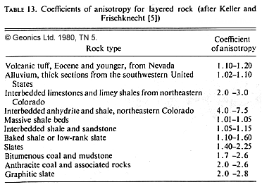
, where ![]() is called the coefficient of anisotropy. See the table below for some values of λ encountered in common geological materials.
is called the coefficient of anisotropy. See the table below for some values of λ encountered in common geological materials.
 |
 |
 One of the fundamental principles regarding current flow is that away from the current electrode, all the current that goes into a body must come out. There are no sources or sinks of current anywhere, except at the current electrode itself.
Because there are no sources or sinks of current in the earth (conservation of charge), the normal component of current density is constant across any boundary where conductivity changes. That is, all of the current that flows into one side of the boundary must flow out the other side. Also, since lines of equal potential in an electric field are perpendicular to current flow, the electric field perpendicular to the normal component of current at the boundaries must also be constant across the boundary. Therefore there are two boundary conditions that must hold across interfaces where conductivity changes:
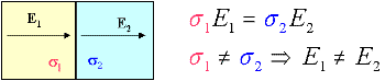
Now, recall that Ohm's law is J = ![]() E. Since the normal component of J is continuous across a boundary where conductivity changes, the normal component of the E-field must NOT be equal. If
E. Since the normal component of J is continuous across a boundary where conductivity changes, the normal component of the E-field must NOT be equal. If ![]() 2 >
2 > ![]() 1 then E2 < E1. The following figure should clarify:
1 then E2 < E1. The following figure should clarify:
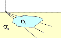
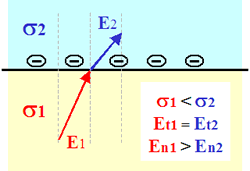
The only way an electric field can change at a boundary is if there is a charge on the boundary. If the current is flowing from a resistive medium to a conductive medium, then the charge buildup will be negative. If the current flows from a conductive medium to a resistive medium, then the charge will be positive. This is illustrated in the diagram below-left, where the anomalous body (blue) is more conductive than the host (yellow). In the figure below-right, the change in E-field is illustrated for a field crossing from a resistive medium (yellow) into a more conductive zone (blue). Tangential components are unchanged, but normal components of E are different so that normal components of J can remain unchanged. This change in direction is the origin of the concept that current lines "converge" upon entering a conductor, and "diverge" upon entering a resistor (illustrated with cartoons of the ore body in this chapter's introduction).
 |
 |
In fact, the charge density that accumulates will be related to the ratio of the two conductivities:
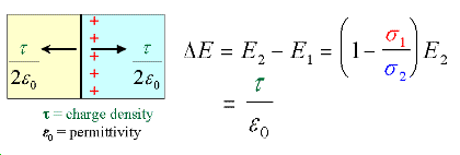
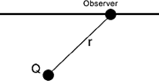 How are charges on boundaries related to DC resistivity surveying? Any electric charge produces an electric potential. The Coulomb electrostatic potential is given by
 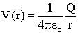 . All charge on the edges of a body produce their own electric potentials, and at the surface (or anywhere else), the total potential is the sum of the potentials due to the individual charges (principal of superposition). These potentials are what we measure as voltages, and they are caused by charges building up on boundaries where conductivity changes, which in turn are caused by the current being forced to flow by the transmitter. Of course we don't measure absolute potential; rather, we measure the potential difference between two locations (say r1 and r2).
 Using the physics and appropriate mathematics to calculate a set of measurements is called "forward modeling." The DC resistivity forward modeling problem involves describing potentials everywhere as a function of conductivity in the ground, geometry, and input current. It requires three fundamental relations:
|
Ohm's law. | |
|
Electric field is the gradient of a scalar potential. | |
|
Divergence of current density equals the rate of change of free charge density. |
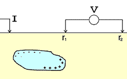
We want to obtain a differential equation and boundary conditions to define the forward problem that will allow us to relate conductivity everywhere to potential everywhere. Start by combining (a) and (b) to say ![]() , then plug this into (c) to get
, then plug this into (c) to get
. (2)
This holds for steady state conditions everywhere, except at the source position (r = rs), where it equals the input current, I. In other words, charge does not accumulate under steady state conditions, except at the point of the source.
Equation (2) can be re-written as
.
The Dirac delta function is used here to indicate that charge density is varying only at the point source of current.
Boundary conditions that must hold are:
This differential equation (4) and the two boundary conditions define the forward problem that relates conductivity everywhere in the ground to potential measured anywhere within or on the surface of the ground.
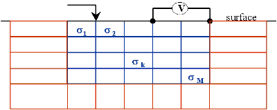
The problem can be discretized for calculation on a computer using finite difference or finite element methods. One approach is given in Dey and Morrison, 1979 (with more details in McGillevry, 1992). Essential aspects of their approach can be summarised as follows:
Equation (4) can also be used directly, resulting in a finite element formulation, as opposed to the finite difference formulation just described. Transformation into the Fourier domain is used here as well.