MeshTools3D: 
User's manual 

Contents

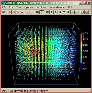
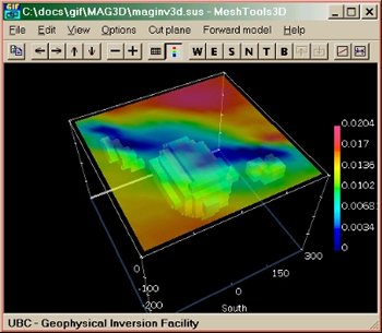
This is MeshTools3D showing vectors for the real part of the H field calculated for a loop source of 1 Amp oscillating at 100 Hz (red square) placed on the surface of an earth with resistivity of 1000 Ohm-m. The air above the earth has nearly zero conductivity. Vector colours represent vector magnitudes, in units of A/m2

Introduction

This UBC-GIF utility has four purposes: 

1. Viewing 3D models of Earth's physical properties that were generated by inversion programs MAG3D, GRAV3D, or DCIP3D;
2. Building 3D blocky models of density or susceptibility, and then running either magfor3d or gzfor3d (requires licensed or educational versions of these forward modelling programs) to generate magnetic or gravity data that would be gathered on a surface above these models;
3. Viewing the 3D distribution of EM fields and EM field components that are generated by EH3D (figure to the right). EM codes are not currently available except to sponsors and colleagues.
4. Viewing 3D models used for calculating SP responses and overlaying various model parameters and data sets to visualize relations between the two. SP codes are not currently available except to sponsors and colleagues.

The program works only with files that are formatted for use by UBC-GIF forward modelling and inversion codes. Models of the earth are specified using two files: a mesh that defines the discretization of the Earth, and a model file that lists the physical property values (or EM field parameters) for all the cells. 

Upon starting the program, read the banner, and respond to the "Open" dialogue by specifying both a mesh and a model file (or 2 models if desired). You could click "Cancel" in this dialogue, then proceed within MeshTools to either create a new mesh (File -> Create mesh ...) prior to building susceptibility or density models for forward modelling, or load an existing model (File -> Open ...). Both the mesh and corresponding physical property (or "model") file must be specified. You can drag-and-drop files from Windows Explorer into the MeshTools "Load Model" dialogue. Two models that are based upon the same mesh can be displayed; see Working with Two Models.

Note that if a file is chosen that is incompatible with the corresponding function, the behaviour of the program can not always be predicted. For example, if a topography file is selected it must be compatible with mesh, models and data (if any) that are in use.

Viewing physical property distributions

Basic Features Start by loading an existing model using File menu Open ... option - recall that you can drag and drop files from Explorer into the file dialogue. Reloading: A model file can be reloaded preserving all view settings via the File | Reload menu. (new 2007) Initial view: The discretized earth is presented with North "into" the screen, in a perspective projection, with the model rotated -65 degrees about the x-axis (angles are positive anti-clockwise when viewing along the axis of rotation, from zero towards positive values of that axis). Zero degrees rotation would result in a top view. Copy images to the Windows Clip Board as a bit mapped image suitable for pasting into any document. Use the Edit menu Copy option, or click the left-most tool bar button. Save images directly as image files - use File menu Save as ... option, and select JPG, PNG, or BMP image formats from the save dialogue's "Save as type" drop down option box (at the bottom of the save dialogue). Mouse behaviour: Note that tooltips appear if the mouse is held over a button for a second or two, and the status bar at the bottom of the window often provides useful information.

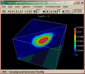
This shows a sliced, isosurface rendered susceptibility model under magnetic data. Several new features are shown:  - label font size is adjustable  - several colour bar styles are available  - Two data sets are plotted, one as a surface map and the second (with elevations) as spheres  - a North arrow is included

• Mouse behaviour continued
  • Left Mouse Button: Click the left mouse button over any model cell and the status bar provides the location and value of the visible location under the cursor. NOTE: this works best if you rotate the volume so that the cell you are looking at has a face that is parallel to the screen. If the volume is a rotated then location and value quantities may not be quite correct.
  • ...OR... Pressing <Ctrl>-Q will toggle the constant display of model coordinates under the mouse cursor.
  • SHIFT-Left Mouse Button: If a cutplane is selected, this moves the cut moves to mouse position. If the mouse is over a blank area (perhaps behind a cut), nothing happens. (new 2007)
  • CTRL-Left Mouse Button: Opens up a dialog box with cell properties. The user can modify cell value. (new 2007)
  • ESC: reverts to a default view with no cuts or isosurfaces.
  • Right Mouse Button: Free hand rotation of the model is achieved by clicking and holding the  right mouse button while moving the mouse anywhere within in the MeshTools window.
  • CTRL-Right Mouse Button:Hold the CTRL key while dragging with the right mouse button to pan the model up & down or side-to-side within the window.
  • Mousewheel moves the cutplane so long as a plane has been defined using the W, E, S, N, T, or B toolbar buttons.
  • Pressing and rolling the mousewheel causes Zoom in/out.
• To reset the view to the opening configuration press "Esc" or select File menu Open, and click the OK button without re-specifying the files.
• The colour bar has no units labelled because the program is not automatically aware of the model type that is being displayed. See also the "rescale" and "min max" options below.
• Output models from GRAV3D are g/cc, so long as data were provided as anomalous gravity in milliGals.
• Susceptibility models are in values of straight S.I. units, so long as data were provided as anomalous total field magnetic field strength in nano Teslas.
• For conductivity models, units are either Ohm-m or S/m.
• For chargeability models, units depend upon what data type was inverted.
• See below for details regarding EM data and fields.
• Use of the arrow keys:
  • up-, down-, left-, right-arrows: rotate the model about the vertical and horizontal axis. Rotation increment is defined using the View menu, Rotation Angles ... option.
  • CTRL + up-, down-, left-, right-arrows: pan the model in the vertical and horizontal directions.
  • SHIFT + up-, down-arrows: When a slicing direction is selected (South, North, East, West, Top, Bottom), the slicing plane is advanced with the SHIFT + up-arrow and retreated with the SHIFT + down-arrow. SHIFT + left-, right-arrows does nothing.
  • ALT + left-, right-arrows: these are used when there are two models being displayed, to fade from one model through to the other.
• Other Keyboard shortcuts
  • <CTRL>-F = Flip colours
  • <CTRL>-Q = toggle the constant display of model coordinates under the mouse cursor.
  • <CTRL>-C = copy image to Windows clip board
  • <CTRL>-O = open new file
  • (SHIFT-C) = Copy plotting parameters
  • (SHIFT-V) = Paste plotting parameters
  • <ALT-1> = decrease labels font size
  • <ALT-2> = increase labels font size
  • r = reset scale
  • m = toggle mesh grid
  • e, w, s, n, t, b = start slicing from east, west, south, north, top, bottom respectively.
  • ESC = reset slicing to display the whole volume.

Overlaying one or more data sets:

• (New 2006) Importing data (or other) files using the File | Load data... This dialogue (right) contains options for how data are displayed.
  • More than one data file can be loaded, and display properties, including whether each data set is displayed, and it's transparency, can be adjusted for each data set.
  • First browse for a data file. Then click "Load".
  • Then browse for a second (and subsequent) data file, and click "Load".
  • Pick one data set using the drop down menu under the "Load" button, adjust plotting method, transparency and colour scale, and check "display" checkbox if the data set is to be visible.
  • Repeat for other data sets.
• The program recognizes any data files in ASCII text format (as well as mag3d and grav3d data files) having three or four columns separated by spaces in the following order (X, Y, Z) or (X, Y, Z, value). Initial rows that are not in the four-column format are ignored.
• When loading a data file, duplicate points get averaged.
• Data can be displayed as contour plots or as points, cylinders, lines or spheres.
• The degree of transparency can be adjusted using the CTRL-left and CTRL-right keys. Note that this is adjusted along with transparency of two models if two models are shown (see below), so viewing data over models is most effective when there is only one model being displayed.
• Also, selecting "colourmap" and clicking "select" allows the data set to be plotted with it's own colour scale.
• NOTE the dialogue box to the right of "plotting method" has a different function depending upon you choice of plotting method.
• Data labels: When plotting data as dots or lines, labels will also be plotted if a 5th column exists in the input data file.
• This File | Load data option makes it easy to include boreholes, transmitters, and other types of information. For example, if a borehole location is to be included, simply build a (X,Y,Z) text file with locations along the borehole. Load this, set the plotting method to "lines", fixt the colour scale to "solid colour" (red for example), set the number of pixels to 2 or 3, and click OK. A line following the points in your text fill will be included within the 3D volume.

Note that use of the File | Load data option is now the way in which EM transmitters are displayed. See Viewing EM Fields below.

Working with two models

See 3 figures to the right by clicking buttons. The line shows SP potential data generated by forward modelling. Two models are displayed on one mesh. 1. Conductivity model, 2. hydraulic head, 3. both shown semi-transparent. The File menu Open option allows two models to be viewed. They MUST be defined using the identical mesh. When two models are loaded, MeshTools3D displays a small information box that reminds the user of how to adjust transparency of the two models Two models occupy the same volume in the viewing window. They are viewed by altering the transparency of each model. Adjust using ALT-left and ALT-right arrow keys to fade from one model through to the other. The MeshTools3D window's title bar (above the menus) changes to indicate which of the two models is most visible. Also, the colour scale displayed shows the model that is most visible. Title and colour scale both switche automatically when transparency fades through 50%.

• Isosurfaces are displayed based upon the first model specified in the File menu Open dialogue. If you want to display isosurfaces based upon the other model you must change the order in which the two appear in this dialogue box.
• Note that when viewing 2 models, the % transparency is displayed on the status bar. (new 2006)

Menus

The File menu  Opening new models; Reloading: A model file can be reloaded preserving all view settings via the File | Reload menu. (new 2007) Constructing a new mesh; Saving the model to a new name (only if the model has been changed); Saving the viewer window's contents to a bit mapped image file in .bmp or .png or .jpg formats; Reading a topography file that is associated with the model. This is used mainly for forward modelling of magnetics and gravity data. At the present there is no method for importing topography information when viewing 3D volumes produced from 1D results of using EM1DFM (using the "em1d3d.exe" command line utility - see the EM1DFM documentation). Loada data: Choose data to overlay on the model and adjust how data is displayed. Several data sets can be displayed, and each can have it's own presentation style (surface, points, cylinders, lines or spheres, and colour scales can be chosen. Cell faces... is an option allowing display of parameters assigned to cell faces rather than cell contents, such as MAG3D and GRAV3D weighting files. The files containing such information are expected to be as described for weighting files in the respective user manuals. (new 2007) Saving or loading meshtools parameters so they can be applied to other models. " Save parameters ..." creates a .mt3d file which contains all the model and view settings, and optionally the entire mesh and model(s) files. This .mt3d file can be associated with MeshTools3D, so that when it is double-clicked, it would be automatically opened with MeshTools3D. (NOTE summer 2005: The save/load parameters is still experimental.)

Edit menu

• Add Blocks is used to build blocky 3D models of a physical property. This is usually used in conjunction with forward modelling (below) of magnetic and gravity data, but can be used to build models of any physical property. See "Building models" below for more details.
• Smooth is used to make blocky models smoother changing cells around boundaries so transitions between regions occures less abruptly.
• Copy parameters (SHIFT-C) saves most viewing parameters (orientation, slice, etc) to the clipboard.
• Paste Parameters (SHIFT-V) takes parameters from the clipboard and applies them to the current MeshTools3D window. These two commands are very useful for quickly making two open windows display their models in identical ways.
• Copy: This puts a bitmap of the MeshTools3D display into the clipboard. This is the easiest way to put copies of the image into a document or image editor. It is the same as "Save Images" described above in "Basic Features".

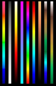
Colour scales left to right: - default - grayscale - colour 2 - colour 3 - colour 4 - colour 5 - colour 6 - topo 1 - topo2

View menu

• There are many options for adjusting the view of the model. These are best explored by trial and error.
• The Reset scale option (also applied simply by typing "r" on the keyboard anytime) changes the colour scale so that is spans the values of cells currently visible on the screen. Change the view of the mesh and press "r" again to set the colour scale to span the new values that are visible.
• Nine different colour maps can be used - they are plotted and listed in the adjacent figure. Scales default and 5 are similar but scale 5 has smaller distribution of green-yellow.
• Font size of labels can be changed (or use <Alt>-<1 | 2> shortcut).
• Details about the mesh itself are provided via the View menu Mesh Stats ... option.
• Obsolete: The Transmitter option is relevant only when viewing EM fields. Use File | Load data to manage a transmitter.
• Options for adjusting the data display are included here (instead of under the "Forward model ,menu", where they were prior to Sept, 2003).

Options menu

• Cutoff ... sets the isosurface level. See Isosurfaces below.
• Min/Max: Allows the colour bar scale to be changed. This feature is important when creating several figures that need to be compared.
• Lights: allows you to select the direction of the "lighting" that is applied to the 3D volume.
• Padding cells: If the model includes padding cells around the core of the Earth model that is of interest, these padding cells can be removed from the display using the Options menu Padding Cells ...option. In the resulting dialogue, enter the number of cells to remove from each side of the cubical model.
• Animate: allows you to generate a set of BMP images (bidmaps) that simulate an animated move between two end members. See "Animations" below.
• Vector properties: allows you to adjust the appearance of vectors used when displaying EM fields. See below for more details.
• Scale Model: permits adjustment of the X Y Z axis scaling (normally set to 1:1:1). This allows you to change the vertical exaggeration, for example.

Remaining menu items

• Cut Plane: see Slicing below.
• Forward Model: see Forward modelling gravity or magnetic data below.
• Help:
  • The About option specifies the version and credits for this program
  • If the the Manual option is selected, the program will attempt to load the file meshtools.pdf from the MeshTools3D.exe directory. If this file is not there the program will attempt to opened the web page at www.eos.ubc.ca/research/ubcgif/documentation/meshtools/meshtools-docs.htm in the user's default browser.
| top |

Seeing inside the volume

There are two principle methods of viewing the inside of models; slicing the volume or specifying an isosurface - Figures and details are provided next.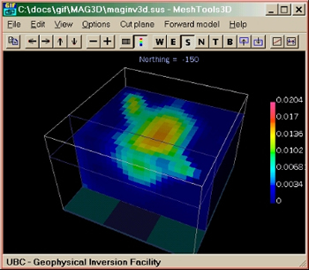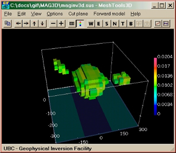

.
Left: Volume imaged by slicing from top and from south. Right: Volume imaged using an isosurface.

Slicing

• Successive layers can be sliced off by holding the SHIFT key down while pressing the UP cursor key, or use toolbar buttons to the right of the W E S N T B buttons.
• Holding down the space bar while moving the cutplane would skip duplicate layers.
• SHIFT-Left Mouse Button: If a cutplane is selected, this moves the cut moves to mouse position. If the mouse is over a blank area (perhaps behind a cut), nothing happens. (new 2007)
• ESC: reverts to a default view with no cuts or isosurfaces.

The SHIFT DOWN key moves the slicing plane back one plane at a time after using the SHIFT UP key. These keys remove or replace successive layers respectively regardless of where you start, so if "Top" is selected, the SHIFT UP key reveals the model values of successively deeper layers. Press the ESC key to revert to an un-sliced view of the model. Diagonal slices can be applied by using the Cut Plane menu Diagonal ... option. Alternatively use the mouse by clicking either of the two right-most tool bar buttons. The last tool bar button permits you to select end points of the diagonal slice using the  right mouse button; instructions appear in the status bar.

Specifying Isosurfaces

An isosurface is essentially a 3D contour surface. MeshTools3D displays an isosurface by not displaying cells with values that are outside specified upper and lower bounds. Use the Options menu Cutoff ... option to define upper and lower bounds. The program will hide values outside these bounds, leaving a 3D "body" that shows the shape of material whose physical properties are within the bounds. The 3D body can be lit in any direction using the Options menu Lights... option, however, the default of "centre" lighting tends to yield the most usable results. Note that isosurface images tend to obscure the fact that models generally consist of smoothly varying physical properties. Two examples showing the same model of magnetic susceptibility are shown below. Pressing the ESC key reverts to a default view with no cuts or isosurfaces.

  .

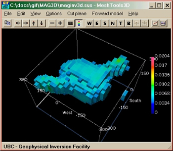
Left: Isosurface specified at 0.01 (scale in SI units) Right: Isosurface specified at 0.005 (scale in SI units)

Viewing EM field distributions

MeshTools3D is also used to view components of the electromagnetic (EM) fields that are generated using the forward modelling program EH3D. In this case the images show distributions of EM field components NOT the distribution of Earth's physical properties. The MeshTools3D program is also used to create the model of Earth's conductivity structure and to place the EM source onto this model (see below), so it is important to stay aware of exactly what is being displayed.

Below left is a figure showing the real part of the magnetic field calculated for a loop source placed on the surface of an earth with resistivity of 1000 Ohm-m. H-vectors are shown in every cell of the model. Vectors along selected planes are shown in separate figures below.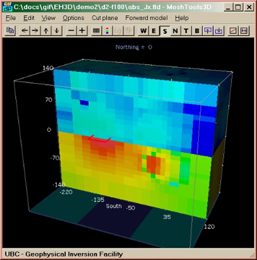

.
 

Unlike earth models, the mesh defined for EH3D calculations includes a substantial volume of air (usually, but not necessarily, equal to the subsurface volume). Air is usually assigned a conductivity of 10^-8 S/m. Complex E and H vectors are generated for every cell (ground and air) in the model domain. The exact location at which each parameter is calculated (cell centre, cell edge, cell face, etc.) is detailed in the EH3D background theory document. Scalar or simple vector parameters must be generated from the complex E or H vectors before EH3D results can be plotted using MeshTools3D. There are 36 scalar parameters and 6 vector parameters that can be generated; see EH3D documentation for a list of these.

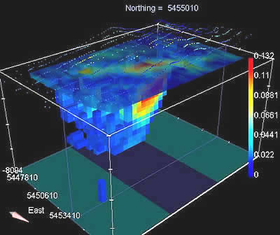
• Once scalar quantities have been generated from raw EH3D output, these will be plotted in the same way as physical property values when MeshTools3D is being used to view an earth model. That is, each cell is given a colour corresponding to the value of the relevant parameter in that cell, according to the colour scale. Units for EM parameters are included in a table in EH3D documentation.
• The figure above right shows the magnitude of current density resulting from a current-loop source. The model volume is sliced along the Y=0 plane, and the ground surface is at the base of the blue colours. In air current density is very small because air is assigned a conductivity of 10^-8 S/m.

Vector parameters initially plotted as small arrows (lines) centred within each cell. All vectors are the same length and their magnetitude is imaged using colour according to the colour scale. This fixed length can be adjusted using the Options menu, Vector properties ... option.  Orientation of the vector in 3 dimensions is correct, and the vector's arrow head is indicated using a small dot coloured to contrast with the background.

(New for 0903) The Options menu, Vector properties ... option permits adjustment of how vectors are displayed. They can be changed to cones (instead of lines), the number of vectors plotted can be reduced by specifying the increment for each dimension, (plot every second vector, every third vector, etc), and the length of the cones or lines can be adjusted. Here is an example of plotting vectors as cones.

Vector data are effectively visualized by displaying only one slice through the model domain. MeshTools3D therefore displays only one plane of mesh cells when a slice direction is chosen (W E S N T or B). Two examples are shown below.

.

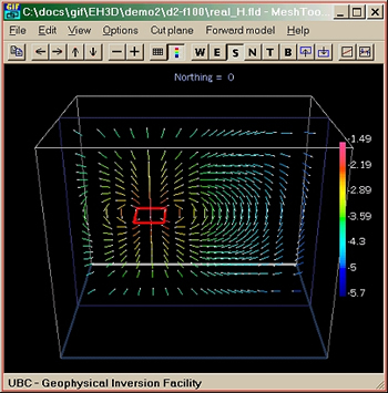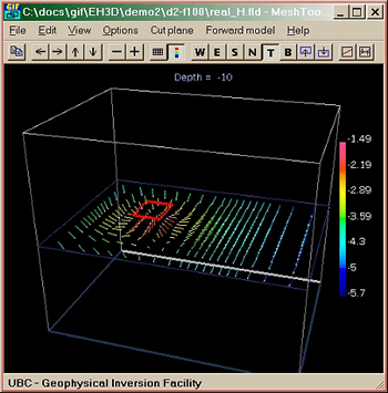Left: Magnetic field vectors (real part) along the Y=0 plane. Right: Magnetic field vectors (real part) along the Z=-10 plane.

All other features (rotation, animation, viewing options, etc.) of MeshTools3D behave in a similar fashion when displaying scalar or vector data. Isosurfaces work as well. Owing to the visual complexity of trying to image a 3D vector field, one effective approach is to specify upper and lower bounds that are quite close to each other. Then you should be able to see a "shell" of vectors without the added confusion of vectors inside and outside that surface. Visually the 3D nature of the field is often enhanced by motion, so use the right mouse button to oscillate or move the image in various ways.

EM sources are plotted in MeshTools3D when the viewer is launched from the EH3D GUI. If you need to view EH3D results that were generated earlier you must start by running the EH3D interface. Open the EH3D control file generated when the previous work was carried out, then check to see that the source is as required in the EH3D GUI's "source type" box. Clicking the "View Fields" button will display those fields generated by the forward calculation specified in the "Label" box, and the source will be visible in the fields plot. Also, clicking any "View" button in EH3D's GUI will display the corresponding synthetic model including the source.

When MeshTools3D is invoked by the EH3DT graphical user interface, the models at each time step specified in EH3DT's "wave.txt" transmitter waveform specification file can be viewed using the "shift->" and "shift<-" cursor keys. The status bar displays the currently displayed model by model number so you must refer to the wave.txt file to correlate model numbers with time steps. A series of time steps can also be exported for animation.

Finally, note that the File | Load data option allows borehole locations, additional transmitters, and other features to be overlayed. See "Multiple data sets" above.

Special Viewing Features

Animations

Versions later than January 2007: Animations of type *.avi are now produced without intermediate *.bmp image files for each frame. Here are steps for creating an animation:

1. Begin by making the Meshtools3d window an appropriate size. Since the animations are created by taking screen captures, the size of the final .avi file will be proportional to the window's area.
2. Position the model. This will be the first frame.
3. In the menu, choose Options | Animation | Start ...
   1. Enter the name of the output .avi file.
   2. A dialog box will appear. Choose the method of creating a movie: "1" or "2".
   3. Enter frames per second. Values from 5 to 15 are usually good.
   4. Click on OK.
4. When method "1" is selected, every time the contents of the window are modified, it will be appended to the movie file.
   1. To duplicate a frame, choose: Options | Animation | Continue, or click the 'a' key.
   2. To end the movie, in the menu choose: Options | Animation | Stop
5. When method "2" is selected, a start and end view is defined and intermediate frames are interpolated:
   1. Position the model to a different view.
   2. In the menu choose: Options | Animation | Continue , or click the 'a' key.
   3. Enter the number of frames to create. Click on OK.
   4. The frames between the start and end views will be interpolated and saved to the movie file.
   5. Repeat the above steps until done.
   6. To end the movie, in the menu choose: Options | Animation | Stop

Notes:

• When creating a movie, try not to obscure the main window with other windows, or you might get some unexpected results.
• Don't forget to "Stop" the movie.
• When recording a movie, you cannot change the window's size.
• If you get an error message just before recording the first frame, it might mean that the movie file with the same name is open by another
  program (Media Player). Close it.
• If you cannot open the movie file with Media Player, it might mean that the movie wasn't "Stop"ed within MeshTools3D.

Versions prior to January 2007: Select the Options menu Animation ... option for instructions to make a series of images that interpolate the view between a specified beginning and end view. The series of bitmap images will be saved in the same directory where the mesh and model files were found. These images must then be converted to an animation using a third party utility. We have used a free command line program called pjBmp2Avi (or Bmp2Avi) from Paul Roberts, available from http://www.divx-digest.com/software/bmp2avi.html as of May 2004. (Use "bmp2avi -?" at the command line for a list of options.) Many other more sophisticated (and probably more expensive) utilities are available via the Internet.

Seeing several models with identical views

To set identical viewing parameters in two or more concurrently running versions of MeshTools3D, first set the desired view parameters for one of the models, then click the Edit menu Copy parameters option in that window, move to the second (and third, etc) MeshTools3D window and click the Edit menu Paste parameters option. This procedure copies viewing parameters such as rotation, slice, etc., but value scales are not copied over. Use the Options menu, Min/max ...option to ensure colour scales are the same for each image.

Building models

Initializing a discretized volume

Start by running the MeshTools3D program. A mesh can be loaded with no model file, or a new uniform mesh can be created using the File menu Create mesh ... option. (See below for notes regarding building models for EH3D.) It is wise to use metres as units to ensure consistency with all modelling and inversion work.

When a new mesh is loaded using the File menu Open option the resulting dialogue has a check box labelled "log". Here's what to do with this check box:

• Leave it blank if you are working with susceptibility or density models. Then the discretized volume will be initialized with all zero values. 
• Check this box if you are working with a conductivity model that will be used for forward modelling with EH3D. You will be given the option to initialize the discretized volume as a halfspace with air (cells above the Z = 0 plane) and ground (cells with Z< 0) having different values. Also, "values" will be displayed in MeshTools3D in log of S/m. 
• NOTE however that model values are never saved in log units regardless of what MeshTools3D is displaying, so never make a conductivity model with cell values in log units.

Adding physical property blocks

To add a buried object to your earth model, select the Edit menu Add blocks ... option, then move the resulting dialogue (see figure to the right) off your viewing area. Also, most users find that a white background is easier to use than the default black background. Finally, recall that you can toggle the mesh view on and off. The following list outlines a procedure for building buried structures.

• Coordinates can be entered in the dialogue box.
• Alternatively the sliders can be used to move blocks and adjust their sizes:
  • First move the single cell that appears to the location of the top, West, North corner of your desired block using the X, Y , and Z sliders. If the cell is not immediately visible moving the sliders will make it appear.
  • Then click the "dx" box, and use the sliders to expand that cell in +X, -Y and +Z directions to create the required shape. The resulting block will approximate an ellipseoid if the "Type=ellipseoid" button is clicked.
  • The three "Slope" controls are used to apply a dip to your structure in either the X or Y directions, or along the XY plane.
• Enter the physical property's value for your feature in the "value: " box. Units should be SI for magnetics, gm/cc for density, and S/m for conductivity (or log S/m if MeshTools3D is currently displaying conductivity in log units - see Initializing ... above). 
• Three buttons and a drop down list in the bottom right are used to add, remove or change the name of blocks.
• NOTE: After clicking OK, you should select the Options menu Min / Max option and click "reset" to generate a colour bar that is correct for the range of physical property values you have defined.
• Be sure do save your model using the File menu Save As ... option.
• As you use the controls, note that the status bar contains information defining the location and size of block you are working on; ie:  .
| top |

Notes regarding building models for EH3D

• The "automatic" mesh is not usually suitable for creating models that will be used for forward modelling EM data using EH3D. You are better off creating your mesh for this program from scratch, then loading this mesh into MeshTools3D to place conductive or susceptible blocks as targets.
• Be sure you understand the difference between the two options discussed above for initializing the discretized volume.
• EM signals decay more slowly in air than in the ground so it is advisable to start with an equal volume of air as ground. Signals are however expected to be small, so this might be relaxed later if you need to reduce the number of cells in the forward calculation. However, you should retain at least several layers of air cells with thicknesses equal to those in the first few layers of your discretized subsurface.
| top |

Forward modelling gravity or magnetic data

The Forward Model menu provides direct access to forward modelling codes supplied as part of the license for MAG3D and GRAV3D inversion programs. The corresponding forward modelling executables must be in the same directory as the MeshTools3D program. When the Magnetics or Gravity options are selected, a dialogue box appears asking for some necessary parameters. The magnetics dialogue is shown to the right, and the gravity dialogue is the same except of course without the three magnetic field specification boxes.

• For magnetics, you must enter the inclination, declination, and total field strength for the location on the Earth where you are expecting this model. Inclination is positive down (northern hemisphere) and declination is positive to the east of the mesh's north. One way of obtaining values for (I, D, F) is to use the JAVA applet (or the similar freeware software) available from most national geological services. Examples (April 2007) are:
  • USGS: On-line magnetic-field model calculator.
  • Canadian Geological Survey: Magnetic field calculator.
  • Or Google something like "gsc magnetic field calculate".
• The four values in the "Data area" specify surface locations where data will be calculated. The default is at the centre of every mesh cell, but it is common to change this so that data look more like survey lines. For example line-spacing may be greater than station spacing. It is also important to keep the data set from being too large for efficient inversion.
• Elevation should be set appropriately for the instrument you are simulating - a sensor height of 2 m above the ground is common for ground-based surveys.

Magnetics or gravity forward code is started as a low priority task on your Windows PC. When you click the OK button, a command line window will appear giving a running tally of how much of the calculation is complete. It will close when the forward calculations are done, and data will be plotted as a semi transparent anomaly map at the correct elevation above the mesh model (see image above).

If the UBC-GIF utilitity  gm-data-viewer is in the same directory as MeshTools3D then a new window showing the data should appear. Use of gm-data-viewer should be self explanatory, but there is a manual for this program. Examine the menu options and the tool button quick hints (hold the mouse over a button for a couple of seconds). Note that the gm-data-viewing plotting tool also lets you examine a line profile anywhere on the data set.

Important: If the synthetic data generated by forward modelling is to be inverted as part of work that is investigating what types of models might arise by inversion, you must remember to add noise to the synthetic data set prior to inverting. This is done within the gm-data-viewer program via that program's Edit menu.

Running MeshTools3D from the command line

If MeshTools3D is run from the command line with no parameters (or by double clicking it's icon) it will open directly with a blank window. However, a model can be loaded directly using the following command line parameters. Only the mesh file is necessary; other parameters are optional. If the model file is not included, MeshTools3D will display the mesh.

Filenames on command line should be in quotes. This allows spaces in filenames.
meshtools3d "mesh file" "model file"
meshtools3d "mesh file" "model file++model2 file"
When the first line of the model file has "models", it can now also contain the number of padding cells removed:
   models nmodels [pad_x1 pad_x2 pad_y1 pad_y2 pad_z2 pad_z1]