GM-data-viewer manual

gm-data-viewer:
User's manual

Most recent update: Feb 2007 (Update history)

gm-data-viewer is a small data plotting program written for the MS Windows™ Operating System by Roman Shekhtman of the UBC Geophysical Inversion Facility (UBC-GIF). Note that the program is not intended to be a sophisticated data plotter - it is a utility to help visualize data sets while working with UBC-GIF modelling and inversion tools.

Installing the program:
Simply extract the executable program from it's archived into any directory on your MS Windows™ computer, and follow the instructions for use.

Input file format

Input data must be in one of three formats. Attempts to feed other types of data files to gm-data-viewer will result in unpredictable behaviour.

The first format is a simple XYZ columns separated by spaces or tabs. No example is given here, but the following notes apply:

Any text following an "!" mark is ignored.
The first line (not including comments) must contain only one integer giving the number of data points in the data set.
Data are listed in the rest of the file with one datum per row. The columns are:
- X-location | Y-location | datum value
Columns must be separated by spaces or tabs
Values can be integer, float, or scientific types, and in any units.
There must be the correct number of data, as identified on the first line (not including comments).
Use the Options menu to adjust the title and axis/scale labels.

The second format is the one used for gravity data sets by UBC-GIF codes. It can also be used for any XYZV data set.

 !comment
 2601
 0 0 1 43.2 4.3 
 0 2 1 41.7 4.2 
 0 4 1 38.6 3.9 
 0 6 1 37.6 3.8
.
.
.

Any text following an "!" mark is ignored.
The first line (not including comments) contains only one integer giving the number of data points in the data set.
Data are listed in the rest of the file with one datum per row. The columns are:
- X-location | Y-location | elevation | datum value | error on datum
Notes on columns:
- columns must be separated by spaces or tabs
- elevations can be plotted in gm-data-viewer (versions following 20060609 - see help menu). Even if you don't have elevations, the column should contain place holders.
- values can be integer, float, or scientific types, and in any units.
- errors are not required, but if present they can be plotted (see below).
There must be the correct number of data, as identified on the first line (not including comments).
By default, plots of data provided in this format will be labelled as "Observed Gravity Data". This can be changed using the Options menu.

The third format is very similar to the second, and it is used by UBC-GIF magnetics data:

 !comment 
 !comment2 
 -10.00 30.00 50000.00 !! incl, decl, geomag 
 -10.00 30.00 !! aincl, adecl: anomaly 
 2601 !! # of data 
 0 0 1 43.2 4.3 
 0 2 1 41.7 4.2 
 0 4 1 38.6 3.9 
 0 6 1 37.6 3.8
.
.
.

Any text following an "!" mark is ignored.
The five numbers in the top two lines are reserved for use in UBC-GIF programs. They are not used by gm-data-viewer except to complete the plot titles, but there must be place holder numbers there for gm-data-viewer to work.
The third line (not including comments) is an integer giving the number of data points in the data set.
Data are listed in the rest of the file with one datum per row. the columns are:
- X-location | Y-location | elevation | datum value | error on datum
Notes on columns - same as "second format" above.
There must be the correct number of data, as identified on the third line (not including comments).
Plots of data provided with this format will be labelled as "Observed Magnetic Data", with inclination, declination, and field strength. This can be changed using the Options menu.

Features

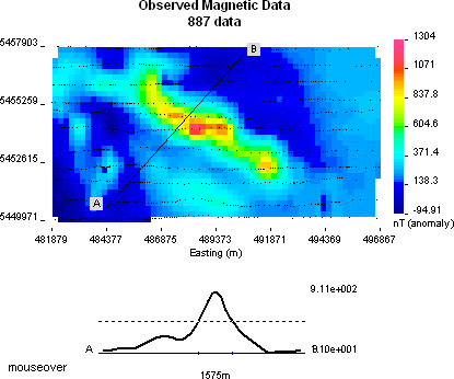
A list of features is given here. See the menu description for more details. The image to the right shows a small magnetic data set.

One or two data sets can be plotted (one is shown to the right). By default the first data set is plotted one above the second, but they can be plotted side-by-side using View => arrangement.
When data are in second or third formats, elevation can be plotted as the second data set using View => elevation, or the right-most toolbar button.
The image can be saved to the Window's clipboard, and then pasted into any other application that can accept a "*.bmp" image (such as a wordprocessor). *.bmp images tend to be large so you are advised to convert to *.gif or *.jpg images or any other formats using a bitmap image editing tool.
Instead of contour plotting, the data can be plotted as dots coloured according to the colour scale. See via mouseover on the figure above.
Contouring: Data do not have to be on a grid, but only a fairly simple triangulation algorithm is used for interpolation onto a grid. This step is automatic. Two types of pixel interpolation are provided, giving either a blocky "pixelated" look, or a smoother appearance (mouseover on this link changes the example).
The image can be enlarged or shrunk (magnify + and - buttons).
Locations of actual data points can be overlayed on the plot as dots (as shown on this image).
By default, the colour scale is labelled mGals if a "gravity" style data set was used, and with nT if a "magnetics" style data set was used. For other types of data, use Options => Labels to change plot and scale titles.
Font size of labels can be changed. (View => font | ...) or <Alt>-<1 | 2>

Colour scales
left to right:

- default
- grayscale
- colour 2
- colour 3
- colour 4
- colour 5
- colour 6
- topo 1
- topo2

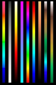The colour map can be either of several built in options via View => Colourmap ... . Try for yourself. There is no option for user-specified colour scales. Available colour maps are shown to the right.

The minimum and maximum values for the colour scale can be adjusted separately for the two displayed data sets.
A sub set (or region) of the data can be specified for plotting (via Options => Region).
Once a region has been selected using Options => Region the data set can be cropped (Edit => Crop) and the reduced data set can be saved.
Data can be decimated (downsampled) using integer values via (Edit => Downsample data ... ). The resulting data reduced set can be saved.
A line profile at any location through the first data set can be generated - shown above, and see below for more details. Click outside the data region to remove the line profile.
A map of the errors specified with the first input data set can be plotted.
The difference between two data sets can be plotted, either directly, or normalized by error values in the first data set. This is usually used to generate a misfit map which compares observed with predicted data during an inversion.
Errors, random noise, and a constant offset can be assigned within the program and the modified data set can be saved.
When the mouse is pointing to a data point, <SHIFT>-<Right mouse button> causes a dialog box to open displaying data information. The user can then change error or delete the data point.
True values of the nearest datum to the mouse pointer are shown in the program's status bar (at the bottom of the window) when the right mouse button is clicked (as shown in the figure above). The datum being seen is highlighted, even when data points are not shown.

Menus

Use of gm-data-viewer menus should be self explanatory. Here are a few tips:

The tool bar duplicates some menu options. Each tool button has a tool tip if the mouse pointer is held over it for a few seconds.
The File menu contains open and save options. In the open dialogue, two files can be specified.
- This was originally included in order to view both measured and predicted data sets while working on a geophysical inversion project.
- The feature is also useful for comparing different data sets that were gathered on identical survey areas.
- NOTE the two data files must be the same type (either "gravity" or "magnetics" data sets, and discussed above).
- The "text editor" option opens the data file in Windows Notepad.
The Edit menu contains the three modify data set options (below). The Downsample option is here, as is the crop option (inactive unless Options => Region was used). It also includes an image copy option which pastes a copy of the display into the Windows clipboard.
The View menu contains options for adjusting display parameters. The Elevation option is only active if the input file is in the second or third formats.
The Options menu contains the scale min / max adjustment, region select and title changing options.

Line profiles

As noted in "Features", and shown in the image above, this plotting tool lets you examine a line profile anywhere on the data set. Click and Drag (using the left mouse button) from the start to the end of any line in any direction, over the contoured data set. The program will label the line's endpoints with A and B, and the graph will appear below the contour plot.

Click anywhere on the graph line of this profile and a horizontal line will appear at that amplitude, with labels on the axis showing the width of the anomaly at that amplitude. Note that if there was a second contour plot, it will be removed from the display when line profiles are created.

Click outside the data region to remove the line profile.

Modifying data sets

Errors can be assigned to all data by specifying a percent and minimum. These will be added to the data set as it's fifth column if the File menu, save option is used.

Random Gaussien noise can be added to the data values by specifying a percent and minimum. Each datum will have random noise added which will be included in the image, and will be saved if the file is saved. Don't save to the original file name or you will loose the original, unchanged data set!

A constant value can be added to all data values. Data will retain this addition if the file is saved.

Single data points can be adjusted (error or value) by pointing to the datum and pressing <SHIFT - Right Button>.

Cropping a data set means throwing away all data outside the area specified using Options => Region . As before, if you save without changing the file name, the original data will be lost.

Downsampling by integer factors can also be done. For example, if "3" is specified (via Edit => Downsample data ... ) every third data point will be kept and all other values will be thrown away.

The command line

Finally, if gm-data-viewer is run from the command line with no parameters (or by double clicking it's icon) it will open directly with a blank window. However, a data set can be loaded directly using the following command line parameters:

gm-data-viewer datafile /pre /pre - read a predicted data file (must be called 'maginv3d.pre' or 'gzinv3d.pre')