|
Geotechnical work also requires quantitative, accurately
located information about the subsurface. Figure 7a. below shows
initial unprocessed results of a DC electrical survey over calcine
tailings at the Sullivan Mine in southern BC. Lateral locations of
conductive material can be interpreted directly. However, for this
application, there was a need to characterize the extent and depth of
the calcine material (which has a higher electrical conductivity than
host rocks) partly to determine the quantity of calcine and partly to
constrain the possible subsurface paths along which ground water could
travel.
Limitations of standard data presentation
The standard form of presentation shown in the top panel
of figure 7, known as a pseudosection, distorts the actual
distribution of subsurface physical properties. Note that no vertical
axis scale is provided. Without formal inversion there is no way to
identify the position and value of electrically conductive or resistive
materials that gave rise to the observed data.
Also, with resistivity surveys it is important to estimate the depth of investigation
because the ability to resolve geology at depth depends upon survey
geometry and subsurface conductivity as well as the current source
power. Traditionally (prior to development of formal inversion
techniques), geophysicists used ad-hoc rules to identify the
depths at which interpretations became unreliable.
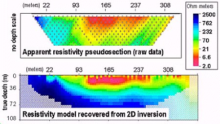 Figure 7: Figure 7:
a. (top) Raw DC resistivity data from a survey over calcine tailings are plotted
in pseudosection format. Resistivity values are apparent rather than true intrinsic
resistivities, and the pattern is determined by the plotting convention. Circles indicate plotting points for recorded
data values. Lateral surface distribution of highly conductive (i.e. low resistivity) calcine
is recognizable, but details of the thickness and geometry of the
conductive zone are obscured.
b. (Bottom) The conductivity
model recovered by 2D inversion of data in the top panel. Each
rectangular cell has the value of it's conductivity determined by the
inversion algorithm. The location and volume of high
conductivity material is clearly defined. The variability at the
surface is due to a thin resistive cover of course bouldery fill
overlying the area. Portions of the 2D model that are not sensitive to the survey are hatched out.
Note that conductivity (which has units of Seimens per metre) is the inverse of resistivity (quoted in units of Ohm-m). |
Depth of investigation
A geophysical survey provides information about a limited volume of the earth. Models produced by inversion usually extend beyond those limits. The value of a physical parameter outside the area of illumination is determined only by parameters in the inversion and does not present reliable information. To prevent over-interpretation of the inversioin results it is best to remove those regions from the final images that are to be displayed. The hatching in Figure 7b accomplishes this goal. It is evident that the geophysical survey provides no information beyond the ends of the survey line, and also the survey's instrument geometry and source energy power results in a limited penetration depth. The maximum depth depends upon the greatest separation of the current and potential electrodes and also upon the level of signal strength compared to noise.
Discussion
There is a well-defined region of high
electrical conductivity (ie low resistivity, in red colours) near the
surface and a region of lower conductivity (blues) that appears at the
surface.
The low conductivity coincides with a known bedrock outcrop and this adds confidence about the interpretability of the image.
Interpretation of a precise depth for the interface
between conductive material and bedrock would be greatly aided by a
single borehole drilled to a depth of roughly 50 metres anywhere within
the high conductivity region. This would also help to identify the value of
conductivity at which the physical interface should be interpreted.
|
