 Goals Goals
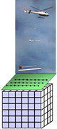
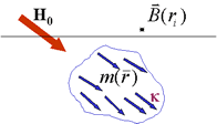
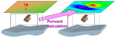
We want to calculate observations of B (magnetic flux density) at any location in three dimensions, for an arbitray 3D distribution of susceptible material, with any orientation of inducing field. This is a general case of the magnetics forward modelling problem. Specific cases that will not be discussed here include calculating fields everywhere due to a solid polygon of susceptible material, and calculating fields of other more constrained geometries. For our more general situation, known parameters will be (1) susceptibility within each cell of a discretized volume of earth, and (2) the geometry of the datum location with respect to each cell. Conceptually, the earth under the surface will be divided into discrete cells, as illustrated in the sketch to the right showing an airborne magnetic survey.
To solve the forward problem for magnetics, two fundamental relations are needed: (i) one of maxwell's equations, and (ii) a relation for the magnetic field due to a dipole expressed in terms of a scalar potential. On this page, the solution will be outlined only. Details of the various steps can be found in texts and references that discuss the theory of potential fields theory and applied geophysics. Some suitable texts are listed a separate references page.
Scalar potential
We start with Maxwell's equation relating magnetic field to current (based upon Ampere's law):
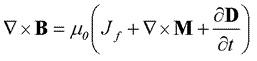 (1). (1).
This equation states that the curl of magnetic field is equal to the vector sum of all moving charges within the region. The Jf is free current density, the second term involves currents related to internal magnetic fields, and the last term accounts for displacement currents.
For geophysical situations we can assume there are no significant currents within the region of interest. Therefore the right hand side goes to zero. Consequently, B is an irrotational field so, according to the Helmoltz theorem, there must be a scalar potential V such that
 (2) . (2) .
Scalar potential due to a magnetic dipole
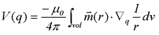
Next we need an expression for magnetic potential at some distance from a small magnetic dipole. Formulate this in terms of scalar potential V(q) at point q some distance from the dipole:
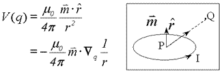 (3). (3).
The magnetic dipole itself can be expressed in either of two ways.
- As an elemental current loop, as shown. Q is the observation location, I is the current in the loop and the m is dipole moment, which is I x surface area, in the direction perpendicular to the loop according to the right hand rule. The rhat is a unit vector in the direction from dipole location towards observation point.
- In terms of a pair of equal but opposite monopoles, the dipole moment is p x ds where p is the monopole strength and ds is the vector distance between them.
More details about this topic, refer to Blakely, pg 72.
B for arbitrary volumes of susceptiblity
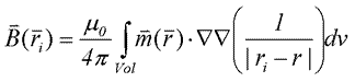
 The magnetic field due to a volume full of dipoles is found by integrating the single dipole expression: The magnetic field due to a volume full of dipoles is found by integrating the single dipole expression:
 (4) . (4) .
Now take the gradient of this scalar potential to find B due to a volume of dipoles:
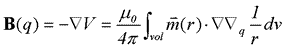 (5) . (5) .
The gradient comes inside since both integration and gradient operators are linear and therefore commutative.
Now we want the magnetic field at any position ri . This is given as a function of a distribution of dipoles, m(r), which in turn is a function of the distribution of susceptibility and inducing field because  (6): (6):
 (7) (7)
 Evidently the magnetic field calculations depend upon Evidently the magnetic field calculations depend upon
- the ambient field strength and direction,
- the distribution of susceptible material below the surface, and
- the position of the measurement.
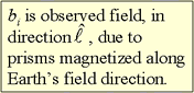
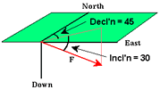
Recall that the ambient field is described in terms of strength, inclination and declination, as shown in the figure to the right.
The discrete version
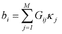
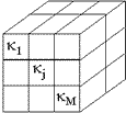 First assume . Also ignore remanent magnetization and self-magnetization. This is valid for most geologic materials because their susceptibility is not very large, but it is not always true. Then discretize the earth into M cells, each with constant k. Now each datum, Bi, will include contributions from all j = 1… M cells: First assume . Also ignore remanent magnetization and self-magnetization. This is valid for most geologic materials because their susceptibility is not very large, but it is not always true. Then discretize the earth into M cells, each with constant k. Now each datum, Bi, will include contributions from all j = 1… M cells:
 (8) (8)
Regarding rectangular discretization, a general earth structure can be adequately modelled if this type of discretization is fine enough. However the problem becomes large very quickly if too many cells are used. For realistic mineral exploration surveys cells that are 25 x 25 x 12.5 metres are usually adequate, although much larger cells are necessary if the survey area is large.
Green's Tensor formulation
We can now conclude by using what we have covered so far on this page to identify the Green’s Tensor formulation for forward modelling:
Each datum bi is a component of the anomalous (induced) B along some direction - for total field measurements this is the direction of the incident field:
 (9) (9)
Pose the problem in terms of susceptibilities using (8);
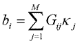 (10) (10)
|
|
where the Gij are calculated by
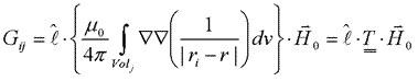 (11) (11)
in which T is called the "Green's tensor". Equation (10) is what we were looking for, namely a forward modelling equation which can calculate measurements anywhere in space caused by a general distribution of susceptible material which is within an ambient (inducing) field with any strength and direction.
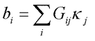
Forward vs Inverse problems
Now we can describe the two fundamental geophysical problem types using these equations.
Forward calculations involve: Given a susceptibility distribution kj = 1, ..., M, and a well-described ambient field, calculate the data bi=1, ..., N.
 or, in matrix form, or, in matrix form,  (12) . (12) .
Inversion involves: Given the data bi , i=1, ..., N, some understanding of their reliability, and a well described ambient field, estimate the susceptibilities kj , j = 1, ..., M such that
 (13). (13).
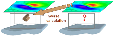
This page is not the place to discuss inversion, but this illustration should provide an initial perspective on how the forward calculations (finding data knowing models) and inversion problems (finding models knowing data and errors) are related.
|