Geophysics foundations:    
Physical properties:  
Electrical resistivity of geologic materials

Introduction

Understanding how electrical resistivity (or conductivity) relates to the actual geologic properties of the earth is important. The following are questions it can help answer:

• If interpretation of a geophysical survey suggested that there is a 10m thick layer of overburden with a resistivity of 11,000 Ohm-m overlying a "basement" with a resistivity of 140 Ohm-m, what geological materials would be consistent with these two layers of different resistivity?
• What if a resistivity profile gathered over an ore body in Australia revealed apparent resistivities ranging from 40 to 600 Ohm-m, while analysis of borehole cores showed that true bulk resistivities range from 80 to >1000 Ohm-m. Are these results consistent, and do they indicated the presence of an economic ore body?
• If bulk resistivity of a deeply buried sandstone is 1000 Ohm-m, can details about the matrix (rock units in which fluids reside) and/or fluid resistivities be extracted? This is of particular interest in hydrogeology, oil and gas exploration and environmental (contaminant) studies.

In this chapter electrical properties of geologic materials are discussed separately for metallic minerals, rocks, soils, and electrolytes (ground fluids).

What is resistivity?

Electrical conductivity (or resistivity) is a bulk property of material describing how well that material allows electric currents to flow through it.

• Resistance is the measured voltage divided by the current. This is Ohm's Law. Resistance will change if the measurement geometry or volume of material changes. Therefore, it is NOT a physical property.
• Resistivity is the resistance per unit volume. Consider current flowing through the unit cube of material shown to the right: resistivity is defined as the voltage measured across a unit cube's length (Volts per metre, or V/m) divided by the current flowing through the unit cube's cross sectional area (Amps per meter squared, or A/m²). This results in units of Ohm-m²/m or Ohm-m. The greek symbol rho,  , is often used to represent resistivity.
• Conductivity, often represented using sigma, , is the inverse of resistivity: = 1/ . Conductivity is given in units of Siemens per metre, or S/m. Units of millisiemens per metre (mS/m) are often used for small conductivity values; 1000mS/m = 1S/m. So 1mS/m = 1000 Ohm-m, since resistivity and conductivity are inversely related.

The electrical conductivity of Earth's materials varies over many orders of magnitude. It depends upon many factors, including: rock type, porosity, connectivity of pores, nature of the fluid, and metallic content of the solid matrix. A very rough indication of the range of conductivity for rocks and minerals is in the following figure.

Figure 2.

The reminder of this section describes factors affecting electrical conductivity of minerals, rocks, fluids in the ground, soils

Electrical conductivity of metallic minerals

Metallic ore minerals are relatively uncommon compared to other crustal materials. However, they are often the target of mineral exploration. Even in small quantities, they can significantly affect the bulk resistivity of geologic materials. Most metallic ore minerals are electronic semiconductors. Their resistivities are lower than those of metals and highly variable because the inclusion of impurity ions into a particular metallic mineral has a big effect on the resistivity. For example, pure pyrite has a resistivity of about 3x10^-5 Ohm-m but mixing in minor amounts of copper can increase the resistivity six orders of magnitude to 10 Ohm-m. Conductivity properties of some important minerals can be summarized as follows:

• Pyrrhotite (FeS) is consistently highly conductive mineral.
• Graphite ( C ) is a true conductor like a metal (i.e. not a semiconductor like ore minerals), and it is very conductive, even in very low concentrations. It is also chargeable (a different physical property - see the separate chapter on Chargeability), and it is notoriously difficult to distinguish from metallic ore minerals.
• Pyrite (FeS₂) is the most common metallic sulfide and has the most variable conductivity. Its conductivity is generally higher than porous rocks.
• Galena (PbS) and magnetite (Fe₃O₄) are conductive as minerals, but much less conductive as ore because of their loose crystal structures.
• Other conductive minerals include Bornite (CuFeS₄), chalcocite (Cu₂S), covellite (CuS), ilmenite (FeTiO₃), molybdenite (MoS₂), and the manganese minerals holandite and pyrolusite.
• Haematite and zincblende are usually nearly insulators.

Although metallic minerals (particularly sulfides) may be conductive, there are at least two reasons why ore-grade deposits of these minerals may not be as conductive as expected.

• Sulfide deposits can be either desseminated or massive. In the first type the mineral occurs as fine particles dispersed throughout the matrix, and in the second, the mineral occures in a more homogeneous form. Desseminated sulfides may be resistive or conductive, whereas massive sulfides are likely to be conductive.
• Chemical and/or thermal alteration can convert metallic minerals into oxides or other forms that are not as conductive as the original minerals.

Soils and rocks are composed mostly of silicate minerals, which are essentially insulators, meaning that they have low electrical conductivity. The most common exceptions include magnetite, specular hematite, carbon, graphite, pyrite, and pyrrhotite. In general, conduction is largely electrolytic, and conductivity depends mainly upon: Porosity, hydraulic permeability, which describes how pores are interconnected, moisture content, concentration of dissolved electrolytes, temperature and phase of pore fluid, amount and composition of colloids (clay content). Figure 4.
Pore space and pore geometry are the most significant factors. Porosity exists mostly in joints, fractures, vugs (dissolved pockets in limestones and dolomites), and intergranular voids in sedimentary rocks. The figure above and tables below (from Geonics TN5, 1980) give some idea of the complexity, and range of porosities possible. The "Ratio" column is bulk resistivity divided by electrolyte resistivity (see Archie's law below).
Vuggy porosity (composed of larger discrete voids) may have very low permeability making for low resistivity when measured using galvanic (DC current) techniques. However, inductively measured resistivity (using electromagentic induction methods) may be higher because currents induced by oscillating electromagnetic fields do not have to flow over large distances. See "Foundations => Survey methods" and "Foundations => Geophysical surveys" for details about these surveying techniques. Resistivity may be anisotropic in layered rocks, especially for shales where the coefficient of anisotropy (ratio of transverse resistivity to longitudinal resistivity) can be as high as 4. See the "Anisotropy" section below for more details.

Electrolytes in the ground

Conductivity of fluids depends upon quantity and mobility (velocity) of charge carriers. Mobility depends on viscosity of fluid (hence temperature) and diameter of charge carriers. Temperature dependence is significant. For sodium chloride solutions, change of conductivity is roughly 2.2% per degree C. So a change of 40^oC doubles the conductivity. In the illustration showing conductivities of waters in the Great Lakes (below), compare conductivities in igneous (western) versus sedimentary (eastern) regions, and note the dependence of conductivity on temperature of these lake waters. 

Natural source	mS/m
Meteoric waters (from precipitation)	1 to 30
Surface waters (lakes & rivers)	0.3 for very pure waters  10,000 for salt lakes  2 to 30 in igneous regions  10 to 100 in sedimentary regions
Soil waters	Up to 10,000  average around 10
Ground water	6 to 30 in igneous regions  1,000 in sedimentary regions
Mine waters (copper, zinc etc. i.e. sulphates)	not usually less than 3,000
Note that Lake Superior is the westernmost lake and therefore in an igneous region, while Lake Ontario is the easternmost or sedimentary region. This may contribute to the generally more conductive waters of the eastern lakes. Figure 5.

The dependence of fluid conductivity on salinity (concentration of ions) for a variety of electrolytes is illustrated to the right. Tap water is usually a minimum of around .01 S/m (i.e. 100 Ohm-m) with a salinity of about 40 ppm, and sea water is roughly 3.3 S/m with a salinity of 30,000 ppm. Compare these values to thoes of lake water shown above. Fluid conductivity depends also upon temperature because the mobility of the ions in solution increases with temperature. This behaviour is opposite to that of metallic conductors which involve electronic conduction rather than ionic conduction, and exhibit resistivity increases with temperature.   Figure 6, adapted from Keller and Frischknecht, 1996.

where R is resistivity, t is temperature, and a is approximately 0.025, where R_18C is resistivity at room temperature (18 degrees C). Recall that resistivity = 1/conductivity.

The effect of porosity  

Saturated clean (no clay) soils or rocks:

Archie's empirical formula relates porosity and water conductivity to bulk conductivity for a variety of consolidated rocks as well as for unconsolidated materials. Archie's formula or "law" is expressed a several ways. One version is  where a is usually 1, _x is bulk conductivity, ₁ is connate ("in place") water conductivity, n is porosity (represented as a fraction of total volume), and m is a constant. A value of m of roughly 1.2 is appropriate for spherical particles, and a value near 1.85 is used for platey particles. This parameter is typically ~1 for unconsolidated materials, 1.4 - 1.6 for sandstones and 2.0 in limestones or dolomites.

An other way of expressing Archie's relation, more commonly used by the oil/gas well-logging industry, is: F=1/^m where F, the "formation factor", is F = Ro/Rw , Ro is bulk resistivity if pore space is filled 100% with brine (connate water), Rw is resistivity of the connate water itself, and is porosity. As always, don't be confused by use of conductivity or resistivity - they are simply reciprocal of each other. It is easy to use a spreadsheet to explore how Archie's equations dictate how porosity and resistivity are related in different materials.

Figure 7.

Unsaturated clean (no clay) soils:

In the funicular zone of soils (figure to the right) moisture does not completely fill pore spaces, but there are still conduction paths. A law similar to Archie's can be used where n is now the fraction of pore volume filled with electrolyte instead of porosity, and m = 2. Using this, conductivity appears to be very small for low moisture contents.

However, the "wetting" of material is critical in affecting conductivity, and slightly wet materials are much more conductive than dry materials. The relation shown below is similar to Archie's formula, and gives water saturation, S_W, in clean (no clay) formations, where  is porosity, _w is resistivity of water, _t is total resistivity, and a and m are both empirically calculated constants. This relation is hard to use, and definitely does not apply to dirty (clayey) material.

Therefore, water saturation may be estimated if

1. electrical methods can be used to find formation resistivity,
2. if connate water can be tested, and
3. if porosity can be estimated.

This is similar to finding water saturation, Sw, when a portion of the pore space is filled with oil or gas, as is frequently done, using well-logging data in hydrocarbon reservoirs.

Resistivity of soils

The electrical conductivity of soils is rather complicated, with many factors affecting the bulk properties. The following material is not covered in most texts on applied geophysics, but it is important because soils are usually (with the exception of borehole work) the closest materials to the survey electrodes. Therefore, soils have a significant effect on results. As noted above, the primary reference is Geonics TN5, 1980.

Porosity ranges from 20% to 70% for most unconsolidated materials (i.e. for soils). However, it is not common to have a large range of porosities in one situation. As noted above, porosity is the primary property related to resistivity, hence the difficulty in distinguishing between sand and gravel with the same porosity.

Effect of freezing on conductivity of soils

Reducing temperature reduces electrolytic activity, and hence conductivity. The figure to the right shows this effect in terms of resistivity. Upon freezing, conductivity of water becomes that of ice, which is very low. However, freezing is rarely simple. Fresh water freezes at a higher temperature than saline water. Therefore solutes tend to become concentrated in a zone of unfrozen saline water adjacent to soil particles. Also, the electric field of cations adsorbed onto soil particles locally orients water molecules near the particle, preventing them from freezing.

The net effect is a slight and steady decrease in conductivity as temperatures approach freezing, then a levelling off through 0 degrees and a further decrease below freezing.

Colloidal conductivity
(conductivity due to clay)

Complexity and variety of soil types is illustrated in the ternary diagram below left. It does not take much clay to change electrical properties of soils. Any fine grained mineral exhibits a certain Cation Exchange Capacity (CEC). That is, charges (cations) can be adsorbed (attached to the surface) onto the slightly negatively charged surface, and these can subsequently be exchanged or dissolved.

Figure 9. US Department of Agriculture textural classification triangle (ternary diagram). Point P is a clay (soil) with 50% clay, 20% silt, 30% sand.  (From Geonics TN-5, 1980).

Figure 10a. Illite (a clay mineral) with total surface area of 100m2/gm (photo Credit: R. Knight.) Figure 10b. Quartz overgrowths in sandstone with total surface area of 0.1m2/gm (photo credit: R. Knight.)

Since clay has a huge surface area to volume ratio, it has a much higher exchange capacity. This is especially the case with the clays vermiculite and montmorillonite. Therefore, clays can dramatically increase the conductivity of connate water, especially fresh waters. Saline waters may not have much more capacity to absorb extra electrolytes.

Anisotropic ground

Anisotropy means "depending upon direction". Structural anisotropy (for example layering or fracturing) may cause the electrical properties of the ground to be anisotropic. This means that measured apparent resistivity will depend upon the direction of the measurement system, as in the adjacent figure. Anisotropy may be very interesting; for example, preferential directions of fluid flow may well be determined by measuring how resistivity varies as a function of the orientation of the measurement electrodes (eg. north-south versus east-west). However, if anisotropy exists but is ignored, then true ground resistivities that are interpreted from measured apparent resistivities may not be correct.

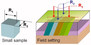For anisotropic materials, R1 NOT equal R2.

Vertically anisotropic ground:
For normal resistivity surveys carried out at the surface, there is no way to tell the difference between resistivity measured vertically and resistivity measured horizontally. Therefore, vertical anisotropy is undetectable at the surface. If such anisotropy exists, depth estimates will be in error by a factor of, λ, the coefficient of anisotropy, defined as λ=(Rv/Rh)^1/2, where Rv and Rh are vertical to horizontal resistivities respectively.

Horizontally anisotropic ground:
Horizontal anisotropy means that resistivity measured with electrodes oriented in one direction will be different from that measured using the same array oriented in a perpendicular direction (eg. "Field setting" in the figure above). In general, "transverse resistivity" (as in R₁ in the figure, measured perpendicular to the bedding plane) will be greater than "longitudinal resistivity" (R₂ in the figure, measured parallel to the bedding plane).

A counter-intuitive effect:
It should be noted that the effect of steeply dipping beds on surface resistivity measurements is not as might be first expected. If anisotropy is steeply dipping (and there is no overburden), one might expect that measured resistivity would be lowest parallel to strike (R₂ in the figure above) since current tends to flow along paths of least resistance. In fact, measured resistivity is highest along strike because of the increased current density parallel to the survey. Apparent resistivity calculations assume uniform current density in three dimensions. When current density is higher than it would be in uniform ground, measured potential difference is higher for the given current source, resulting in a higher apparent resistivity. Therefore resistivities measured with arrays placed along strike are over-estimated and resistivities measured perpendicular to strike are under-estimated. 

Why anisotropy occurs:
For readers wanting more rigourous treatment, here is an explanation of how structural anisotropy (for example layering or fracturing) causes the simple form of Ohm's law to become insufficient. Because current flow is not necessarily parallel to the forcing electric field, the simple form of Ohm's law,   , must be re-written as  

;

where J is vectoral current density, J_i is the i^th component of current density, E is the electric field vector, V is voltage and _ik is the ik^th component of a conductivity tensor. In homogeneous ground with single current and potential electrodes, the expression for V in terms of resistivity and distance from the current source is . In anisotropic ground there are both horizontal and a vertical resistivities. The expression for voltage in terms of the horizontally and vertically oriented resistivities and distance is where  is called the coefficient of anisotropy (introduced above under "Vertically anisotropic ground"). See the table to the right for some values of lambda encountered in common geological materials.

Aspects of soil formation affecting electrical properties of soils

It is worth discussing the formation of soils in order to gain a better appreciation for what is involved when predicting electrical properties of near-surface materials, and when interpreting shallow geophysical surveys. This discussion does not replace a course on soil science, but some issues that affect electrical resistivity should become clearer. Generally, electrical properties are affected by varying clay content, ion type and ion concentration in water. The following is an outline of how these factors evolve in soils.

Weathering involves mechanical, chemical and biological processes that convert surficial materials to humus (organically derived matter), clay and fine-grained sediments. In the presence of water and CO₂ rocks are broken down into ions (often dissolved and removed by drainage), clay minerals are formed, water is used up (becomes part of clay compounds), and solutions become more basic (i.e. less acidic). The process is self perpetuating since a thin layer of soil will cause the relevant processes to occur more rapidly at the rock surface. This is because the layer retains water and CO₂ which produces weak carbonic acid, which combines with rock components to form clays.

Speed of weathering is a function of temperature, vegetative growth, and availability of moisture. Therefore tropical soils tend to be thick. Well drained soils tend to be devoid of unstable minerals (i.e. electrolytes), and dry soils tend to be saline (therefore conductive). The figure at the right is a typical soil profile. The A zone is typically intensely weathered, permeable and devoid of solutes. The B zone is generally much tighter (less porose), richer in clays (both local and transported from A ), and controls how much water gets to the C zone and underlying rock layers. The C zone is generally permeable, and consists of less-weathered parent material. The D zone is often treated as non-porous and impermeable.

Figure 11.

Figure 12.

Soil moisture is affected by several factors. Refer to Figure 7 above:

• In the pendular zone, water exists in isolated rings around tight spots. In the funicular zone, there is a thin layer of water over the surface area. Thickness of this depends on capillary forces.
• If there is fine grained material over coarse layering, the fine grained region may have funicular water, while the coarse layer may have pendular water, and may therefore have a lower conductivity.
• Behaviour of the water table depends upon many things including permeability (which ranges by a factor of 10¹⁰ !), and regional humidity, as sketched in Figure 12 to the right. These factors can cause many kinds of water table configurations, some of which may be rather counter-intuitive.

NOTE : these processes discussed here are natural. In the presence of constructed material, surficial layering may be totally different.

References

• Palacky, G.V. (1987), Resistivity characteristics of geologic targets, in Electromagnetic Methods in Applied Geophysics, Vol 1, Theory, 1351
• Geonics Ltd. Technical Note 5 (1980), Electrical Conductivity of Soils and Rocks, technical references (see the references page).
• Keller, G.V., and Frischknecht, F.C., (1996) Electrical methods in geophysical prospecting, Pergamon, London.