Geophysics foundations:    
Quick overview:  
EM terrain conductivity

General concept

Electromagnetic methods involve using oscillating electromagnetic energy which penetrates the ground and causes (induces) secondary EM fields in regions of elevated electrical conductivity. Terrain conductivity surveys usually involve a handheld instrument operating at a single frequency. Some systems estimate terrain conductivity at several frequencies. One transmitter coil generates the EM energy and a second receiver coil detects EM fields caused by the transmitter as well as fields induced in subsurface conductive regions. The combination of EM fields which is seen by the receiver is a signal that is not generally in phase with the transmitted sinusoidal signal. Therefore the received signal can be thought of as consisting of two parts, one which is in phase with the transmitter (called the in phase component) and the other which is 90 degrees out of phase (called the quadrature or quad phase). These two terms are used in explanations below.

Large data sets can be collected efficiently but results can not be used directly to learn about variations with depth. Data are usually plotted as maps or line profiles of apparent conductivity and interpreted to find the ground positions directly above conductive features. Note that terrain conductivity mapping is a special case of frequency domain electromagnetic methods.

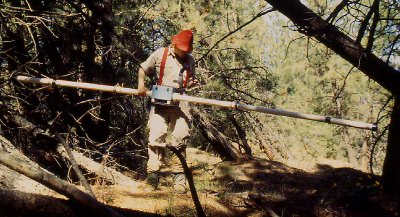
EM-31; a special case of terrain conductivity The Geonics EM-31 instrument is used to map average variations of electrical conductivity at depths between zero and three to six metres. Rapid acquisition of spatially dense data sets is usually the most important requirement. When searching for discrete targets, the most important design consideration is to avoid spatial aliasing (defined in the glossary) . For small 3D targets (such as buried drums), a tightly spaced grid would be required. For 2D targets (such as buried utility pipes), data spacing along profile lines would likely be tighter than spacing between lines, assuming lines can be placed perpendicular to the target orientation.

Mapping electrical conductivity of the ground

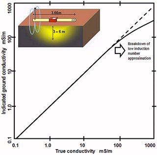
The estimation of ground conductivity is carried out using an approximation formula that relates the quad phase measurement to the conductivity of the ground. The formula is valid for the so-called "low induction number" situation; that is, when the coil spacing is much smaller than skin depth (defined in the glossary) of EM signals at the frequency being used. The EM-31 provides a good approximation for true ground conductivity when that conductivity is less than roughly 1000 mS/m. As the true conductivity of the ground becomes larger than 1000 mS/m, the value provided by the EM-31 becomes more of an underestimate. The figure to the right illustrates this. Details can be found in technical note TN-6 on the Geonics website.

These comments about terrain conductivity hold when the ground within range of the instrument is uniform. In non-uniform ground the instrument yields a value called the "apparent conductivity," which is a complicated weighted average of conductivities of all materials within range. The inset image to the right illustrates with a fading yellow zone how the effect of ground causes the total result to decay at greater distances from the instrument.

Response to "long" or "small" targets

Long targets (called 2D targets) have one dimension much larger than the instrument's coil spacing and the other dimension much smaller. Examples include pipes, trenches, etc. "Small" targets, such as small metal objects have all dimensions smaller than the coil spacing. For 2D targets, the patterns on response curves or maps depends upon whether the 3.66m long instrument boom is oriented parallel or perpendicular to the target. This is because the geometry of source fields, induced currents in the target, and the sensing receiver, is different for the two situations. Both the quadrature phase (apparent conductivity) and in-phase responses depend upon orientation. Click the buttons below to see the orientation and response for these two configurations. Boom perpendicular to targets. Boom parallel to targets. Both parallel and perpendicular data sets. The response to small objects will look similar to that of 2D objects, except that the orientation of the instrument boom does not make any difference. The response to small buried metal targets will be more evident on the in-phase measurements than the quad phase (apparent conductivity) measurements.